Basics
Tutorials
Models
Inference
Verification
Theory
Waveform likelihood with waveform model uncertainties
Using the heron likelihood function
In order to allow Bayesian inference to be conducted using the heron model a new likelihood function is required which is able to incorporate the waveform uncertainty in the likelihood estimate.
The heron.likelihood function contains suitable likelihood functions for incorporation into sampling engines.
CUDALikelihood
The CUDA Likelihood function allows the GPU on a system to be leveraged to perform likelihood calculations, and should be used with models which use the heron.models.torchbased.CUDAModel base class.
This likelihood function allows considerable acceleration compared to a CPU-based likelihood function, since the waveform is both generated and correlated on the GPU.
-
class
heron.likelihood.CUDALikelihood(model, data, window, asd=None, psd=None, start=None, device=device(type='cuda'), generator_args={})[source]¶ A general likelihood function for models with waveform uncertainty.
- Parameters
model (
heron.model) – The waveform model to use.data (
elk.waveform.Timeseries) – The timeseries data to analyse.window (
torch.tensor) – A tensor defining the windowing function to be applied to data and the model when an FFT is performed.asd (
heron.utils.Complex) – The frequency series representing the amplitude spectral density of the noise indata.
Examples
>>> import torch
>>> import elk
>>> import elk.waveform
>>> from .utils import Complex
>>> generator = HeronCUDAIMR()
>>> window = torch.blackman_window(164)
>>> noise = torch.randn(164, device=device) * 1e-20
>>> asd = Complex((window*noise).rfft(1))
>>> signal = generator.time_domain_waveform({'mass ratio': 0.9},
                          times=np.linspace(-0.01, 0.005, 164))
>>> detection = Timeseries(
       data=(torch.tensor(signal[0].data, device=device)+noise).cpu(),
       times=signal[0].times)
>>> l = Likelihood(generator, detection, window, asd=asd.clone())
>>> l({"mass ratio": 0.5})
Theory
This section details the derivation and the behaviour of the matched-filtering likelihood function for heron waveform models.
The approach taken to derive this is closely related to the approach described in [MooreBerryChuaGair16], however we do not take the approach of adding a statistical waveform difference to an existing approximant, and instead use a statistical model which produces the waveform as a statistical distribution.
Given measured data \(d(f)\) which is composed of some signal \(s(f)\) and stationary Gaussian noise \(n(f)\) which has a power spectral density \(S_n(f)\) [MooreColeBerry15], that is
then we can perform matched filtering to analyse the signal \(s(f)\) using some waveform model \(h(f,\vec{\lambda})\).
For convenience from this point forward we define \(s \gets s(f)\), and \(h(\vec{\lambda}) \gets h(f, \vec{\lambda})\).
From Bayes Theorem
where \(p'(s|\vec{\lambda})\) is the likelihood that the signal \(s\) is a realisation of the model \(h(\lambda)\).
This likelihood is then
which introduces the noise-weighted inner product of two vectors,
with \(\kappa\) labelling the \(M\) frequency bins witha resolution \(\delta f\).
The models we use for the gravitational waveform are known to be imperfect, however if we imagine a perfect waveform, we can define a likelihood function \(p(s|\vec{\lambda})\) which represents this model. For a good approximate model then \(p(s|\vec{\lambda}) \approx p'(s|\vec{\lambda})\).
The conventional approach to improving this agreement is to seek ever better approximate models. The approach outlined in [MooreBerryChuaGair16] works by modelling the difference between the “true” likelihood and the approximate one using Gaussian process regression.
Here we take a third approach.
Each waveform drawn from the Heron model is a draw from a probability distribution; given the probabilistic nature of the waveform it is necessary to include the probability of the waveform in the likelihood function, and then marginalise this out as a nuisance parameter, that is
The expression for \(p(h(\vec{\lambda})\) for the heron model is analytic, by virtue of it being a Gaussian process.
Letting \(h \gets h(\lambda)\),
with \(\mu \gets \mu(\vec{\lambda})\) and \(K \gets K(\vec{\lambda})\) respectively the mean and the covariance matrix of the Gaussian process evaluated at \(\vec{\lambda}\) for a set of frequencies \(f_1 \cdots f_M\). For convenience we can introduce the notation \((x|y)\) for the inner product weighted by the model variance.
The full likelihood expression is then the integral of the product of Gaussians, which is analytical, giving
Implementation
- MooreColeBerry15
C. J. Moore, R. H. Cole, and C. P. L. Berry. Gravitational-wave sensitivity curves. Classical and Quantum Gravity, 32(1):015014, January 2015. arXiv:1408.0740, doi:10.1088/0264-9381/32/1/015014.
- MooreBerryChuaGair16(1,2)
Christopher J. Moore, Christopher P. L. Berry, Alvin J. K. Chua, and Jonathan R. Gair. Improving gravitational-wave parameter estimation using Gaussian process regression. \prd , 93(6):064001, March 2016. arXiv:1509.04066, doi:10.1103/PhysRevD.93.064001.
The production of the likelihood for the heron model goes through a number of steps, given that the waveform model itself works in the time-domain, but the standard method of calculating the likelihood uses a frequency-domain representation.
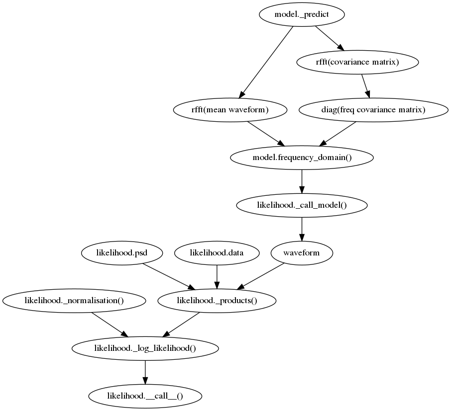
The time-domain waveform, and associated covariance matrix are